Basic Examples

3x2pt for pure \(C_\ell\):

We will calculate the full 3x2pt covariance matrix in harmonic space by running the covariance code with the in config_3x2pt_pure_Cell.ini in the /config_files directory. To obtain a good understanding, we will go through the .ini file section by section:

[covariance terms]
gauss = True
split_gauss = True
nongauss = True
ssc = True

These settings ensure that all terms in the covariance are calculated, that is the Gaussian, non-Gaussian and super-sample covariance terms. The option split_gauss = True results into a further splitting of the Gaussian term into sample-variance, mixed and shot-noise terms in the list output.

[observables]
cosmic_shear = True
est_shear = C_ell
ggl = True
est_ggl = C_ell
clustering = True
est_clust = C_ell
cstellar_mf = False
cross_terms = True
unbiased_clustering = False

Clearly we have switched on all observables and choose C_ell as the required summary statistic. Furthermore, unbiased_clustering is False since a bias model will be used to describe the clustering. Since we do not require the stellar mass function, it is set to False. Setting cross_terms = True ensures that all cross-covariances between the observables are calculated.

[output settings]
directory = ./output/
file = covariance_list.dat, covariance_matrix.mat
style = list, matrix
list_style_spatial_first = True
corrmatrix_plot = correlation_coefficient.pdf
save_configs = save_configs.ini
save_Cells = True
save_trispectra = False
save_alms = True
use_tex = False

This section specifies the output setting and is in general pretty self-explanatory. It should be said, however, list_style_spatial_first = True will lead to the spatial index, \(\ell\) in this case, to vary fastest in the list output. Furthermore, save_alms = True ensures that the suvey modes of the SSC term are saved on disk if a mask file is specified. use_tex = False is just for cosmetics of the output plot, only switch it on if LaTeX is installed.

[covELLspace settings]
delta_z = 0.08
tri_delta_z = 0.5
integration_steps = 500
nz_interpolation_polynom_order = 1
mult_shear_bias = 0, 0, 0, 0, 0

ell_min_clustering = 2
ell_max_clustering = 1000
ell_bins_clustering = 10
ell_type_clustering = log

ell_min_lensing = 2
ell_max_lensing = 5000
ell_bins_lensing = 15
ell_type_lensing = log

Here are the most important settings for the \(C_\ell\): covariance, apart from a few accuracy settings the multipole ranges for clustering and lensing are specified. It should be noted that GGL always assumes the binning for clustering due to the galaxy bias. Here the code will assume 10 equidistant bins (in log) between multipoles 10 and 1000. Note that the centre of the first bin is therefore not \(\ell = 10\). The averaging over the multipoles is carried out internally. mult_shear_bias specifies the values for the multiplicative shear bias uncertainty. Note that, if one uses input \(C_\ell\) which contain already residual shear bias uncertainties, this should be set to zero. Here we deal with 5 lensing bins and therefore specify 5 values.

[survey specs]
survey_area_clust_in_deg2 = 1100
n_eff_clust = 0.16, 0.16
survey_area_ggl_in_deg2 = 1100
survey_area_lensing_in_deg2 = 777
ellipticity_dispersion = 0.270211643434, 0.261576890227, 0.276513819228, 0.265404482999, 0.286084532469
n_eff_lensing = 0.605481425815, 1.163822540526, 1.764459694692, 1.249143662985, 1.207829761642

In this section the survey specifications are passed. We do not pass any mask file, so the survey area is just given in square degrees and the SSC term will use a circular mask with that area to calculate the response. n_eff_clust, n_eff_lensing and ellipticity_dispersion must always match the number of redshift bins passed in the redshift section.

[redshift]
z_directory = ./input/redshift_distribution
zclust_file = BOSS_and_2dFLenS_n_of_z1_res_0.01.asc, BOSS_and_2dFLenS_n_of_z2_res_0.01.asc
value_loc_in_clustbin = left
zlens_file = K1000_photoz_1.asc, K1000_photoz_2.asc, K1000_photoz_3.asc, K1000_photoz_4.asc, K1000_photoz_5.asc
value_loc_in_lensbin = left

Here the file paths of the redshift distributions are specified, both for clustering and lensing (note that in the literature clustering is often refereed to as lenses, or lens distribution, while lensing is referred to as sources or source distribution). The number (or structure) of these files will determine the number of tomographic bins for clustering, lensing and GGL. The clustering signal will always be calculated for all unique bin combinations, even if there is no overlap between the clustering bins. value_loc_in_... specifies how the redshift values in the files should be interpreted, i.e. whether they correspond to the left, mid or right location of the redshift distribution histogram.

[cosmo]
sigma8 = 0.8
h = 0.7
omega_m = 0.3
omega_b = 0.05
omega_de = 0.7
w0 = -1.0
wa = 0.0
ns = 0.965
neff = 3.046
m_nu = 0.0

The cosmology section just specifies the used cosmology, nothing surprising here. astropy is used for background calculations and hmf for the mass function and camb for matter power spectra.

[bias]
bias_files = ./input/bias/zet_dependent_bias.ascii

In this case the bias section is very simple as we are just passing a redshift dependent bias as stored in a file. You should make sure that the bias file covers the same redshift range as the redshift distribution files, otherwise extrapolation will be used. Furthermore, make sure that the bias file structure matches the number of clustering bins.

[IA]
A_IA = 0.264
eta_IA = 0.0
z_pivot_IA = 0.3

The base alignment model in the OneCovariance code is the NLA model and it is implemented such that the alignment signal is always a linear response to the non-linear tidal field. Hence non-Gaussian and SSC terms will also contain a small IA contribution.

[halomodel evaluation]
m_bins = 900
log10m_min = 6
log10m_max = 18
hmf_model = Tinker10
mdef_model = SOMean
mdef_params = overdensity, 200
disable_mass_conversion = True
delta_c = 1.686
transfer_model = CAMB
small_k_damping_for1h = damped

This section defines the parameterswhich are required for halomodel evaluations and usually do not need any modifications.

[powspec evaluation]
non_linear_model = mead2020
HMCode_logT_AGN = 7.3
log10k_bins = 200
log10k_min = -3.49
log10k_max = 2.15

Here the matter power spectrum parameters are defined. Note that the wavenumber range might be updated internally depending on the multipole range. non_linear_model specifies the nonlinear model used for the power spectrum and takes the same keywords as camb and thus cosmosis.

[trispec evaluation]
log10k_bins = 100
log10k_min = -3.49
log10k_max = 2.
matter_klim = 0.001
matter_mulim = 0.001
small_k_damping_for1h = damped
lower_calc_limit = 1e-200

Specifies a few parameters for trispectrum calculation (if the non-Gaussian covariance is required), such as the wavenumber range on which it is evaluated. Note that it will always be inter- and extrapolated onto the required wavenumber range for the projections.

[tabulated inputs files]
Cell_directory = ./input/Cell
Cgg_file = Cell_gg.ascii
Cgm_file = Cell_gkappa.ascii
Cmm_file = Cell_kappakappa.ascii

For this case, we want to use external angular power spectra for the Gaussian covariance. These are passed from the directory ./input/Cell for all required tracers. Make sure that these have the correct format, otherwise the code will complain.

[misc]
num_cores = 8

Lastly, we are running the whole code on 8 cores. Running

python3 covariance.py config_files/config_3x2pt_pure_Cell.ini

Will then execute the covariance and produce some terminal outputs notifying the user about the current process. As output two files will be generated. First the covariance_list.dat containing all elements in a long list:

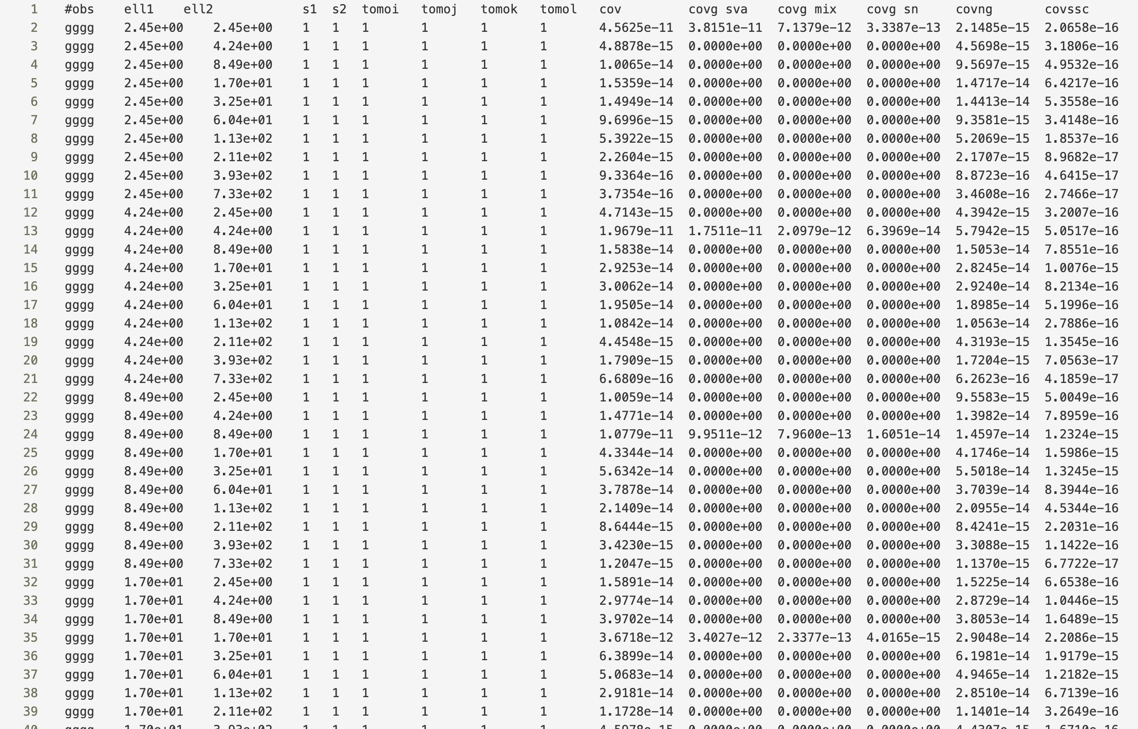
Since split_gauss = True was specified, the Gaussian terms are splitted into the different contributions. The first column labels the tracers, column 2 and 3 the spatial variable, 4 and 5 are the stellar mass sample bins (which is just one since no HoD was used) and column 6-9 label the tomographic bin combination associated with the tracers. The cov column is the final covariance. The Gaussian covariance would be the sum of the columns covg sva, covg mix and covg sn, labeling sample variance, mixed term and shot noise respectively. covng is the non-Gaussian covariance and covssc the super-sample covariance. 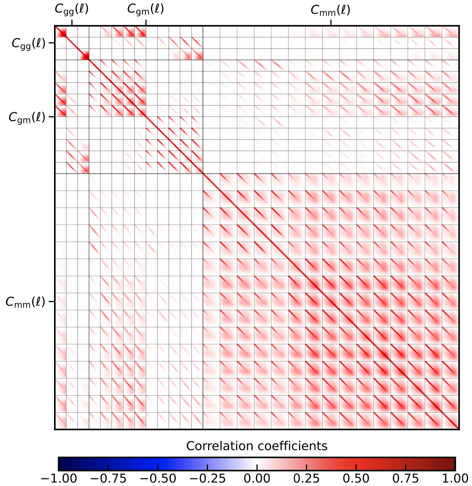Furthermore, a matrix file, covariance_matrix.mat is produced whose general shape is described in the header and can generally be deduced by looking at the plot, correlation_coefficient.pdf.

3x2pt for bandpowers, \(\mathcal{C}_L\):

Repeating the same exercise as in the previous section but now we use bandpowers. To this end one just has to modify the observable section and switch all estimators to bandpowers

[observables]
cosmic_shear = True
est_shear = bandpowers
ggl = True
est_ggl = bandpowers
clustering = True
est_clust = bandpowers
cstellar_mf = False
cross_terms = True
unbiased_clustering = False

Furthermore we have to add the covbandpowers settings section to the config for which we choose:

[covbandpowers settings]
apodisation_log_width_clustering = 0.5

apodisation_log_width = 0.5
theta_lo = 0.5
theta_up = 300
ell_min = 100
ell_max = 1500
ell_bins = 8
ell_type = log

theta_binning = 300
bandpower_accuracy = 1e-7

Defining the multipole range in complete analogy to the \(C_\ell\). The angular range is specified by theta_lo and theta_up with an apodisation log-width of apodisation_log_width to avoid unwanted oscillations in the integration kernels. theta_binning just defines the number of points for the spline of the shot-noise integrals and bandpower_accuracy defines the relative accuracy of the integration. The multipole range and apodisation can also be passed with a subscript _lensing and _clustering again as for the \(C_\ell\). If the settings are passed like this, we assume the same multipole bins for cosmic shear, GGL and clustering. You will also note that in the covariance terms section we changed

split_gauss = False

This leads to a speed up in the calculation since all terms Gaussian terms are calculated at ones and also SSC and non-Gaussian terms are added before being projected. The resulting plot can be seen here:

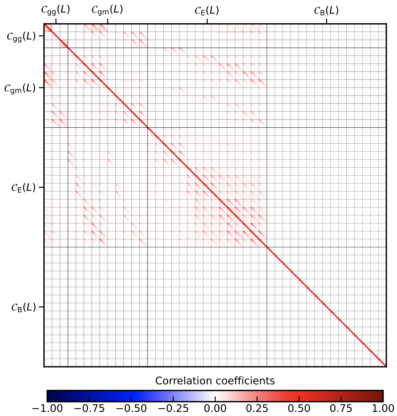
Note that, in contrast to the pure \(C_\ell\), the B-mode is included in the covariance as there can be leakage of E-modes into the B-modes.

3x2pt for realspace correlation functions, \(w(\theta),\; \gamma_\mathrm{t}(\theta),\; \xi_{\pm}(\theta)\):

Next in line are the realspace correlation functions: \(w(\theta),\; \gamma_\mathrm{t}(\theta),\; \xi_{\pm}(\theta)\). It should be noted that, due to their very broad kernels, As a general word of caution: in particular of \(\xi_{-}(\theta)\), they are influenced by highly non-linear scales. The covariance code integrates contributions until the integral does not change by more theta_binning \(1e^{-4}\) (at least by default). For a \(\theta_{\mathrm{min}} =0.5\;\mathrm{arcmin}\) multipoles up to \(\ell\sim 40000\) are required to reach the desired precision. On the other hand, however, \(\xi_{-}(\theta)\) contains quite a bit of the E-mode signal.

In any case, we just switch switch on realspace correlation functions by setting the observables section to

[observables]
cosmic_shear = True
est_shear = xi_pm
ggl = True
est_ggl = gamma_t
clustering = True
est_clust = w
cstellar_mf = False
cross_terms = True
unbiased_clustering = False

as done already in config_3x2pt_rcf.ini. We also add the covTHETAspace settings section and specify two :math:\theta ranges. Again, omitting the _clustering or _lensing will just specify a single angular range.

[covTHETAspace settings]
theta_min_clustering = 50
theta_max_clustering = 300.0
theta_bins_clustering = 5
theta_type_clustering = lin

theta_min_lensing = 1
theta_max_lensing = 300.0
theta_bins_lensing = 8
theta_type_lensing = log

xi_pp = True
xi_mm = True
theta_accuracy = 1e-3
integration_intervals = 40

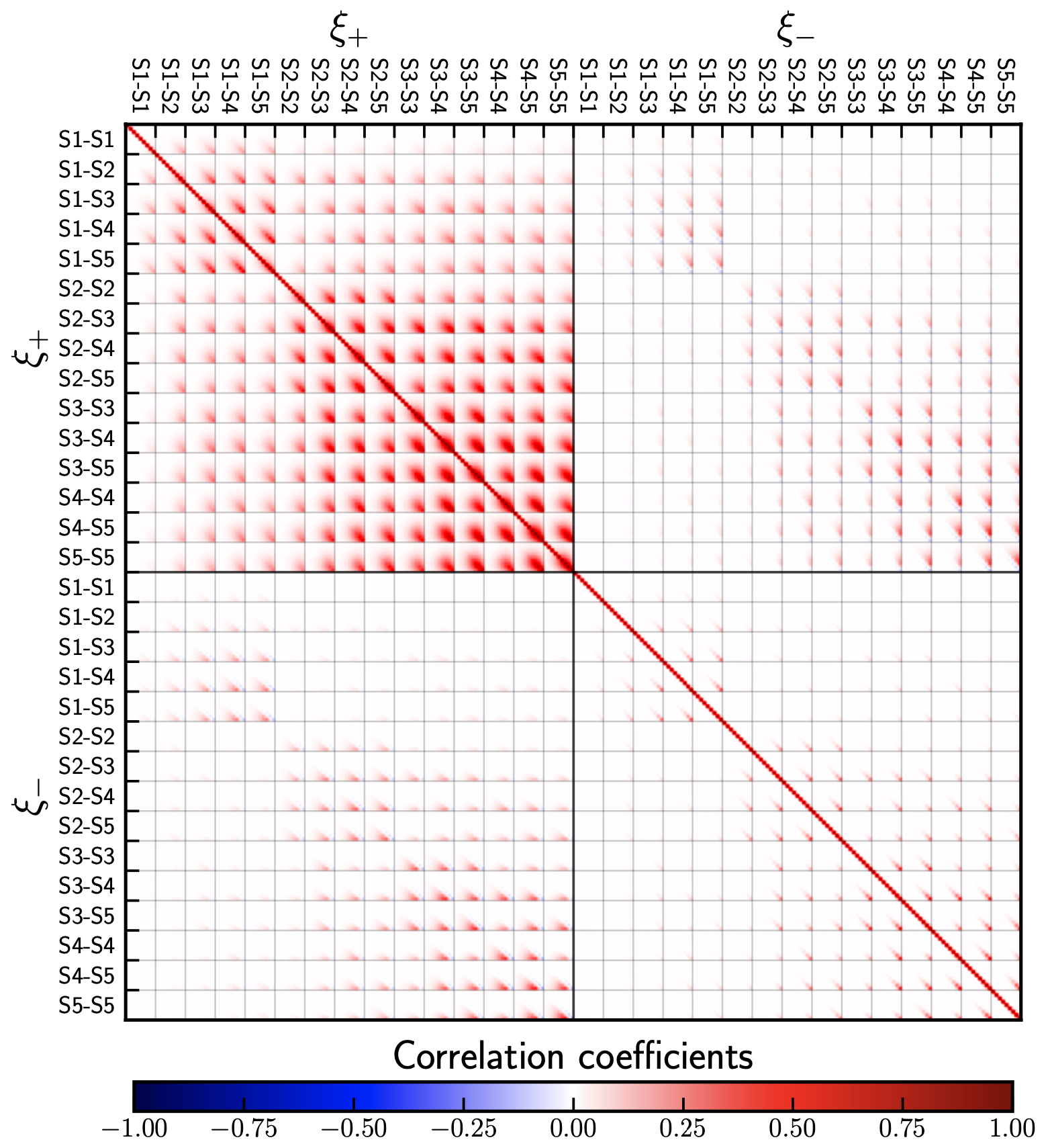
Due to the discussed issues with \(\xi_{-}(\theta)\) there exists the option to remove \(\xi_{-}(\theta)\) from the computation by setting xi_mm = False which speeds things up significantly. However, we will keep it here. Again, we show the resulting correlation coefficient

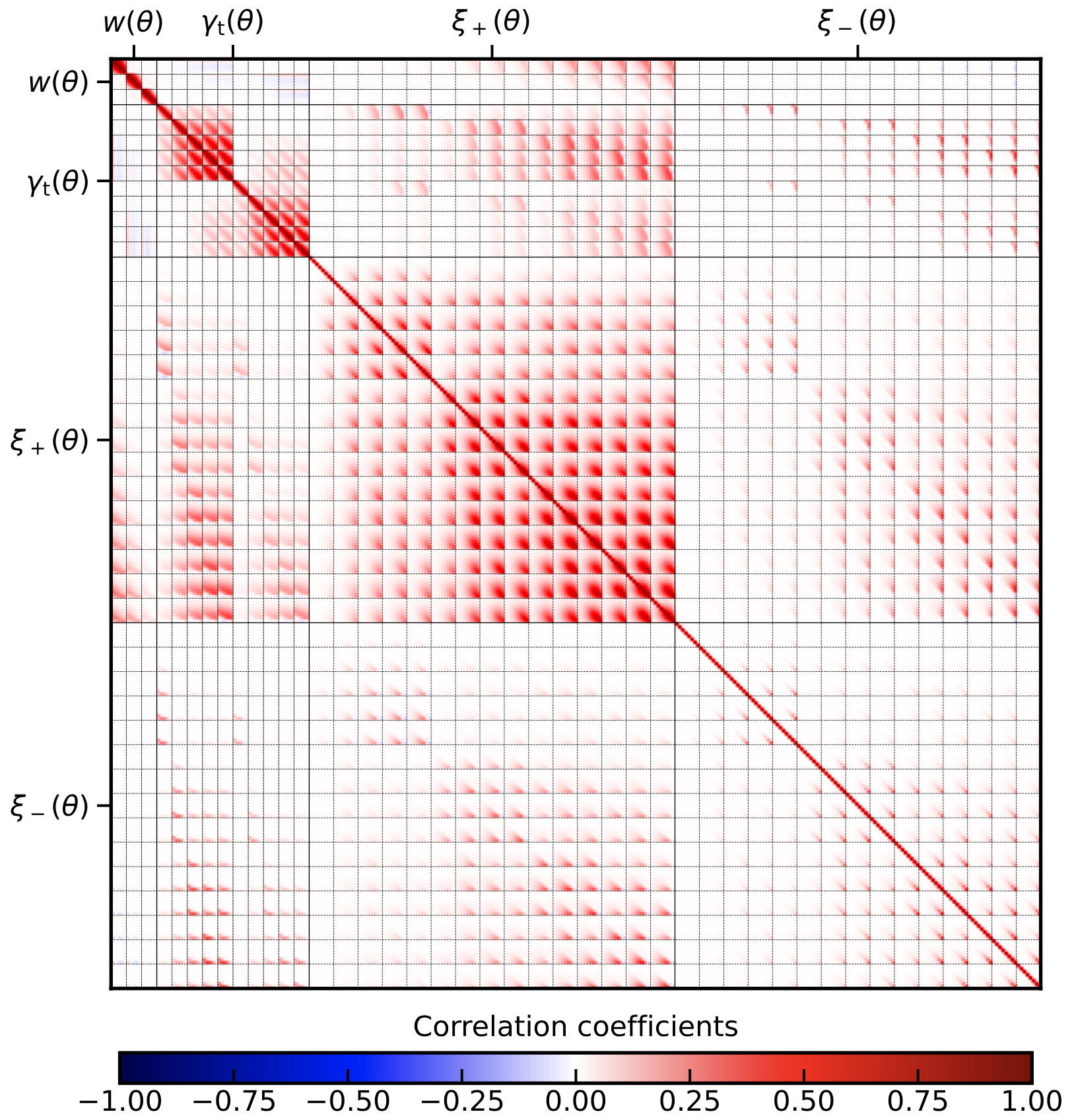
Here we can clearly see that the \(\xi_{-}(\theta)\) covariance is not almost just pure shot noise as it is in the case of bandpowers. That being said, it is still very shot-noise dominated and the variable integration_intervals = 40 can be increased to increase computational speed. For KiDS-1000 we tested this up to integration_intervals = 400 without significant changes in the result.

3x2pt for COSEBIs and \(\Psi\)-stats:

The last summary statistic are COSEBIs and their GGL and galaxy clustering equivalent \(\Psi\)-stats. In this example we only compute the Gaussian covariance terms, so in the config we set:

gauss = True
split_gauss = True
nongauss = False
ssc = False

Specifying the COSEBIs works very similar, all estimators in the observable section are set to cosebi and the following section is added:

[covCOSEBI settings]
En_modes = 5
theta_min = 0.5
theta_max = 300
En_accuracy = 1e-4

For the variables En_modes, theta_min and theta_max there exist, in full analogy to the other summaries, equivalent variables with _clustering and _lensing. With the setting choosen now, they are assumed to be equal. Again, running the covariance code yields the following plot along with the list and amtrix outputfile as before:

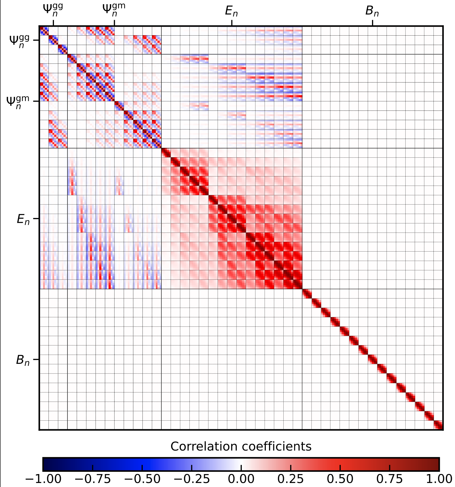
Combining different summary statistics

Since we now know how to run with the standard settings, we can get a bit more adventureous and calculate the covarinace matrix between different summary statistics. To this end we switch on the arbitrary summary section via:

[arbitrary_summary]
do_arbitrary_obs = True
oscillations_straddle = 20
arbitrary_accuracy = 1e-5

This will overwrite the estimators set in the observables. However, you still have to specify the tracers required. Next, the corresponding files for the weight functions need to be added to the tabulated inputs files section. The OneCovariance code requires the following structure for arbitrary summary statistics:

\[\begin{split}\mathcal{O}_{\mathrm{g}_1\mathrm{g}_2}(L) =&\; \int\frac{\ell\mathrm{d}\ell}{2\pi} W^\mathrm{gg}_L(\ell) C_{\mathrm{g}_1\mathrm{g}_2}(\ell) \\ \mathcal{O}_{\mathrm{g}_1\mathrm{m}_2}(L) =&\; \int\frac{\ell\mathrm{d}\ell}{2\pi} W^\mathrm{gm}_L(\ell) C_{\mathrm{g}_1\mathrm{m}_2}(\ell)\;,\end{split}\]

for galaxy clustering and galaxy-galaxy lensing respecitvely. For cosmic shear the situations is slightly different due to its spin-1 structure. We assume that there is no intrinsic B-mode signal in the pure angular power spectrum covariance. However, we allow for B-mode leakage in the summary statistic:

\[\begin{split}\mathcal{O}_{E,\mathrm{m}_1\mathrm{m}_2}(L) =&\; \int\frac{\ell\mathrm{d}\ell}{2\pi} W^\mathrm{mmE}_L(\ell) C_{\mathrm{m}_1\mathrm{m}_2}(\ell) \\ \mathcal{O}_{B,\mathrm{m}_1\mathrm{m}_2}(L) =&\; \int\frac{\ell\mathrm{d}\ell}{2\pi} W^\mathrm{mmB}_L(\ell) C_{\mathrm{m}_1\mathrm{m}_2}(\ell) \;,\end{split}\]

note that \(C_{\mathrm{m}_1\mathrm{m}_2}(\ell)\) is the theoretical E-mode signal. In order to aacurately account for the shot-noise contribution which itself is most accurately computed in real space, we also require the mapping of the summary statistic from realspace:

\[\begin{split}\mathcal{O}_{\mathrm{g}_1\mathrm{g}_2}(L) =&\; \int{\theta\mathrm{d}\theta} R^\mathrm{gg}_L(\theta) w_{\mathrm{g}_1\mathrm{g}_2}(\theta) \\ \mathcal{O}_{\mathrm{g}_1\mathrm{m}_2}(L) =&\; \int{\theta\mathrm{d}\theta} R^\mathrm{gm}_L(\theta) \gamma^{\mathrm{g}_1\mathrm{m}_2}_\mathrm{t}(\theta) \\ \mathcal{O}_{E,\mathrm{m}_1\mathrm{m}_2}(L) = &\; \int{\theta\mathrm{d}\theta} R^\mathrm{mm+}_L(\theta) \xi^{\mathrm{m}_1\mathrm{m}_2}_+(\theta) \\ \mathcal{O}_{B,\mathrm{m}_1\mathrm{m}_2}(L) = &\; \int{\theta\mathrm{d}\theta} R^\mathrm{mm-}_L(\theta) \xi^{\mathrm{m}_1\mathrm{m}_2}_-(\theta)˜;.\end{split}\]

It is now up to the user to provide the files for the weights: \(W^\mathrm{gg}_L(\ell), ...\). In the directory input/arbitrary_summary/script_weights/ there are scripts to generate these weight functions for the most commonly used summary statistics, but you can of course add your own. Now we just have to pass the corresponding files to the code. For this navigate to the tabulated input files (see the file config_3x2pt_arbitrary_summary.ini) and add:

[tabulated inputs files]
arb_summary_directory = ./input/arbitrary_summary/

arb_fourier_filter_gg_file = fourier_weight_realspace_cf_gg_?.table
arb_real_filter_gg_file = real_weight_realspace_cf_gg_?.table

arb_fourier_filter_gm_file = fourier_weight_bandpowers_gm_?.table
arb_real_filter_gm_file = real_weight_bandpowers_gm_?.table

arb_fourier_filter_mmE_file = Wn_0.5_to_300.0_?.table
arb_fourier_filter_mmB_file = Wn_0.5_to_300.0_?.table
arb_real_filter_mm_p_file = Tp_0.5_to_300.0_?.table
arb_real_filter_mm_m_file = Tm_0.5_to_300.0_?.table

In this case first specify the directory where all the filter \(W^\mathrm{gg}_L(\ell), ...\) and \(R^\mathrm{gg}_L(\theta), ...\) are stored and then we specify the filenames: arb_fourier... corresponds to \(W\) and arb_real... corresponds to \(R\). The ? labels the spatial index which is looped over by the code for all files with the specified structured filenames. In this case we use realspace correlation functions for galaxy clustering (measured at 9 theta bins), badpowers for GGL (measured at 8 multipole bins) and COSEBIs for cosmic shear (measured for 5 modes). Note that the corresponding scales over which the 2-point summaries are measured are implicit in the weight functions. You can always rerun the scripts for these weights for different settings. Running the code with config_3x2pt_arbitrary_summary.ini then gives the following output:

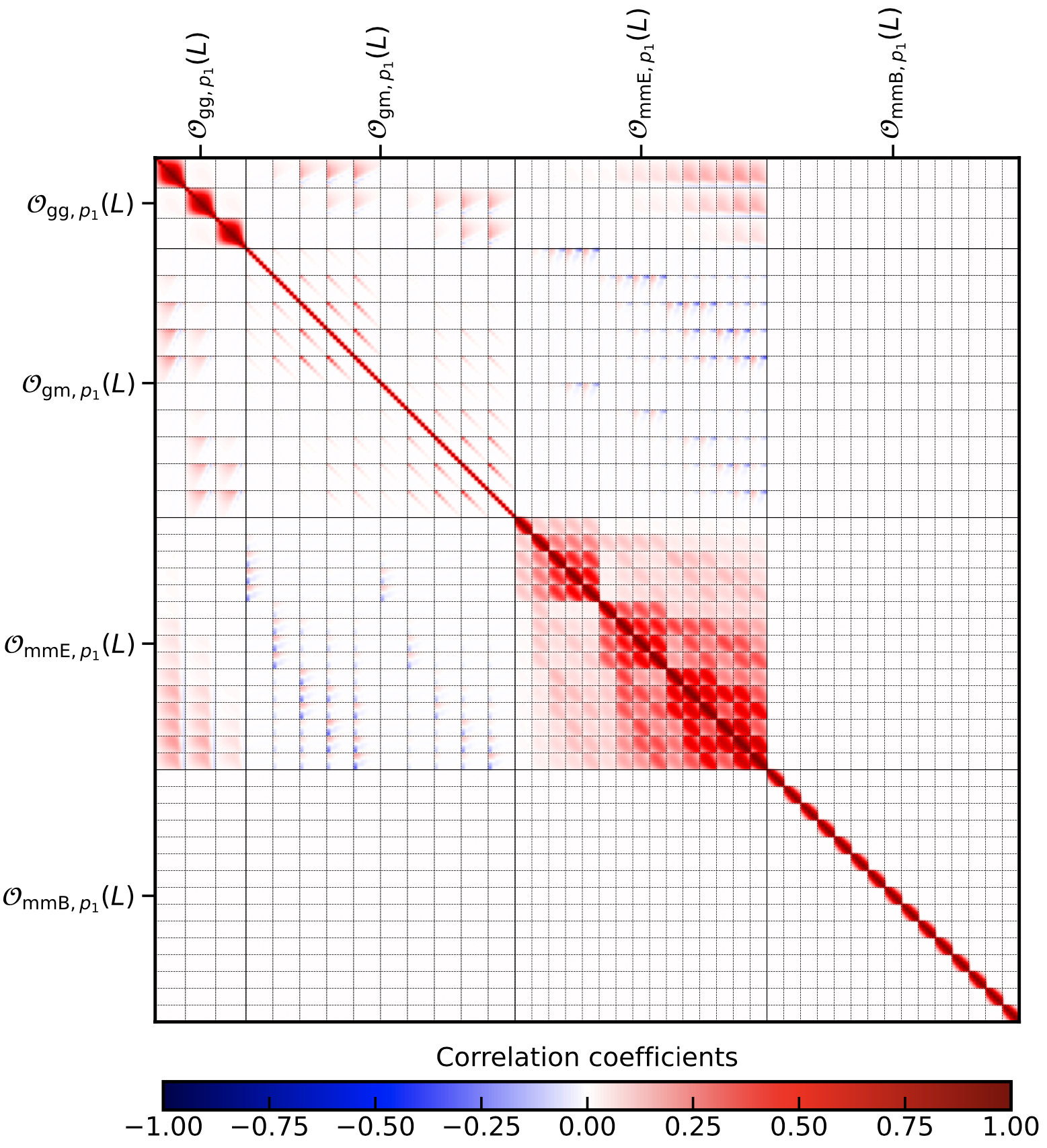
The labelling in the list output is the following: for each tracer, one can define a maximum of two summary statistics, we call them A and B. Next, galaxy clustering will be named gg, galaxy-galaxy lensing gm and cosmic shear mmE, and mmB for whatever is passed in the filter files respectively. So if you pass the \(\xi_\pm\) filters, mmE would correspond to \(\xi_+\). The observable collumn in the list output is then always a pair of this naming scheme, so for example: gg_summary_A_gg_summary_A, the first summary statistic passed for galaxy clustering. The spatial index of the summary statistic will simply be labeled by indices of each of the summary files.

KiDS-1000 covariance

The standard config.ini (after you pulled the directory) will run a simplified KiDS-1000-like cosmic shear setup. Not all parameters specified in the config.ini are used and it is merely used as an explanatory file to explain all the parameters which can be set. Let us take a closer look at the output: Since a plot for the correlation coefficient was requested, we have:

With the corresponding covariance saved in covariance_matrix.mat. A complete list of all the entries can be found in the covariance_list.dat file as shown below.

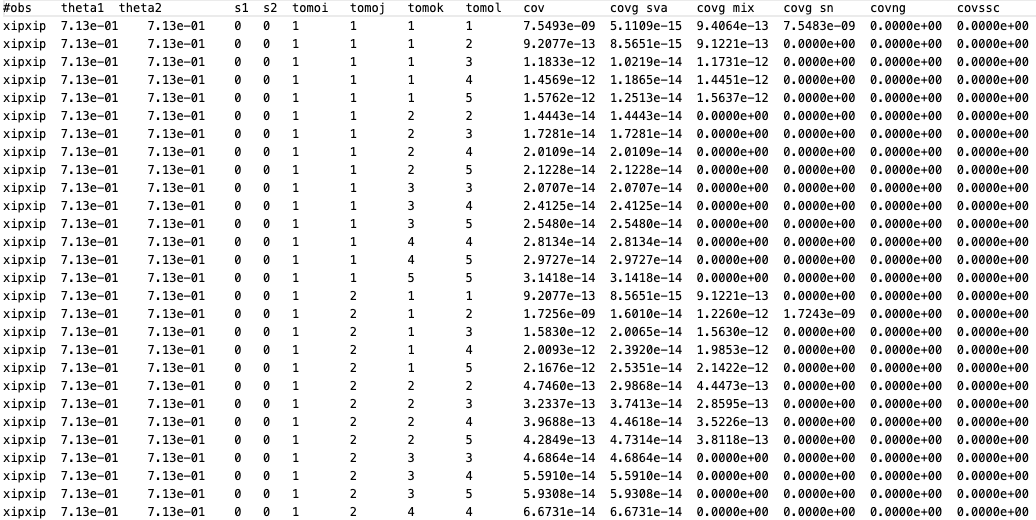
The first column specifies which combination of observables is considered, in this case \(\xi_{+}\xi_{+}\). The second and third column label the combination of the independent spatial variable of the corresponding summary statistic, here this are the two \(\theta\) bins. For bandpowers this would be the multipole bands and for COSEBIS the order. s1 and s2 label the sample bins in mass used (for the evaluation of the halo model integrals). tomoi, …, tomol are the tomographic bin combinations, which start counting at 1. The total covariance is safed in the column cov. If in the config.ini the variable split_gauss is set to true the Gaussian component of the covariance is split into a sample-variance, shot/shape noise and mix term labeled covg_sva, covg_sn and covg_mix respectively. Finally the last two columns show the non-Gaussian and the super-sample covariance term respecitvely, since they have been switched off in the ini-file they are set to zero.

We can calculate the covariance also for bandpowers and COSEBIs by setting:

est_shear = bandpowers

est_shear = cosebi

in the ini-file. Similarly the non-Gaussian and the super-sample covariance term can be requested by setting

nongauss = True

ssc = True

Using Input \(C_\ell\)

In the directory input/Cell files for precomputed angular power spectra, \(C_\ell\), are provided. They should explain the required structure and can be passed to the code by setting

Cell_directory = ./input

Cgg_file = Cell_gg.ascii

Cgm_file = Cell_gkappa.ascii

Cmm_file = Cell_kappakappa.ascii

in the ini-file. In this way one can use the code to produce the covariance of the implemented summary statistic for any tracer for which a harmonic covariance has been calculated.

Selecting tomographic bins

By default, the OneCovariance code calculates all unique combinations of tomographic bins and writes it out into the final matrix file. However, it is often the case that people only want to consider particular bin combinations, this can be done by the variables combinations_clustering, combinations_ggl and combinations_lensing in the observables section. If they are not set, the code falls back to the default for the respective tracer. So for example if you want to only consider the auto-correlations for clustering and you specified 2 redshift files for clustering you might do this by writing:

combinations_clustering = 0-0,1-1

The code will still calculate all combinations. However, it will produce an additional matrix file with your_matrix_file_name_reduced.mat with only the specified tomographic bins.

6x2pt analysis for \(C_\ell\)

The file config_6x2pt_pure_Cell.ini in the directory config_files illustrates how to caclulate the covariance matrix in a \(6\times 2\) analysis. The main feature the OneCovariance is allows to have different binning schemes (and survey areas) for the photometric and spectroscopic clustering samples respectively. We can activate this mode by navigating to covELLspace settings in the configuration file and set the variable:

n_spec = 2

This will tell the code that the first two bins which are passed in the redshift section are treated as spectroscopic and the remaining bins as photometric. The corresponding bins in multipoles can be specified as follows:

ell_min_lensing = 30
ell_max_lensing = 500
ell_bins_lensing = 15
ell_type_lensing = log

ell_spec_min = 10
ell_spec_max = 500
ell_spec_bins = 6
ell_spec_type = log

ell_photo_min = 10
ell_photo_max = 700
ell_photo_bins = 8
ell_photo_type = log

ell_spec_photo_min = 100
ell_spec_photo_max = 500
ell_spec_photo_bins = 12
ell_spec_photo_type = lin

which should be pretty self-explanatory. The values ell_min and ell_max etc. are used for interpolating the \(C_\ell\) covariance. The code will rebin it accordingly in the desired bins. The variables ell_spec_photo_min etc. corresponds to the definition of the \(\ell\) binning if a spectroscopic and a photometric sample are involved in an observable, e.g. photometric cross spectroscopic clustering but also for GGL with a spectroscopic sample as lenses. Furthermore, since we have now effectively three clustering measurements and to GGL ones, we have to specify the respective areas accordingly:

survey_area_clust_in_deg2 = 1100,777,777
survey_area_ggl_in_deg2 = 777,777

The expected order here is the following: for survey_area_clust_in_deg2 it is spec \(\times\) spec, spec \(\times\) phot and phot \(\times\) phot, while GGL expects spec \(\times\) sources and phot \(\times\) sources. The same order translates to the mask files if you want to pass some. Lastly, by default the spectroscopic cross spectroscopic clustering signal will only put out the auto-correlations. However, if redshift space distortions are taken into account in the corresponding redshift distributions, there might be some overlap and adjacent bins can contain some information. This can be enabled by settings

adjacent_clustering_bins = True

Which will then use also the adjacent bins for spectroscopic cross spectroscopic clustering. Running the code in the \(6\times 2\) mode will only produce the matrix output. The corresponding correlation coefficient looks as follows:

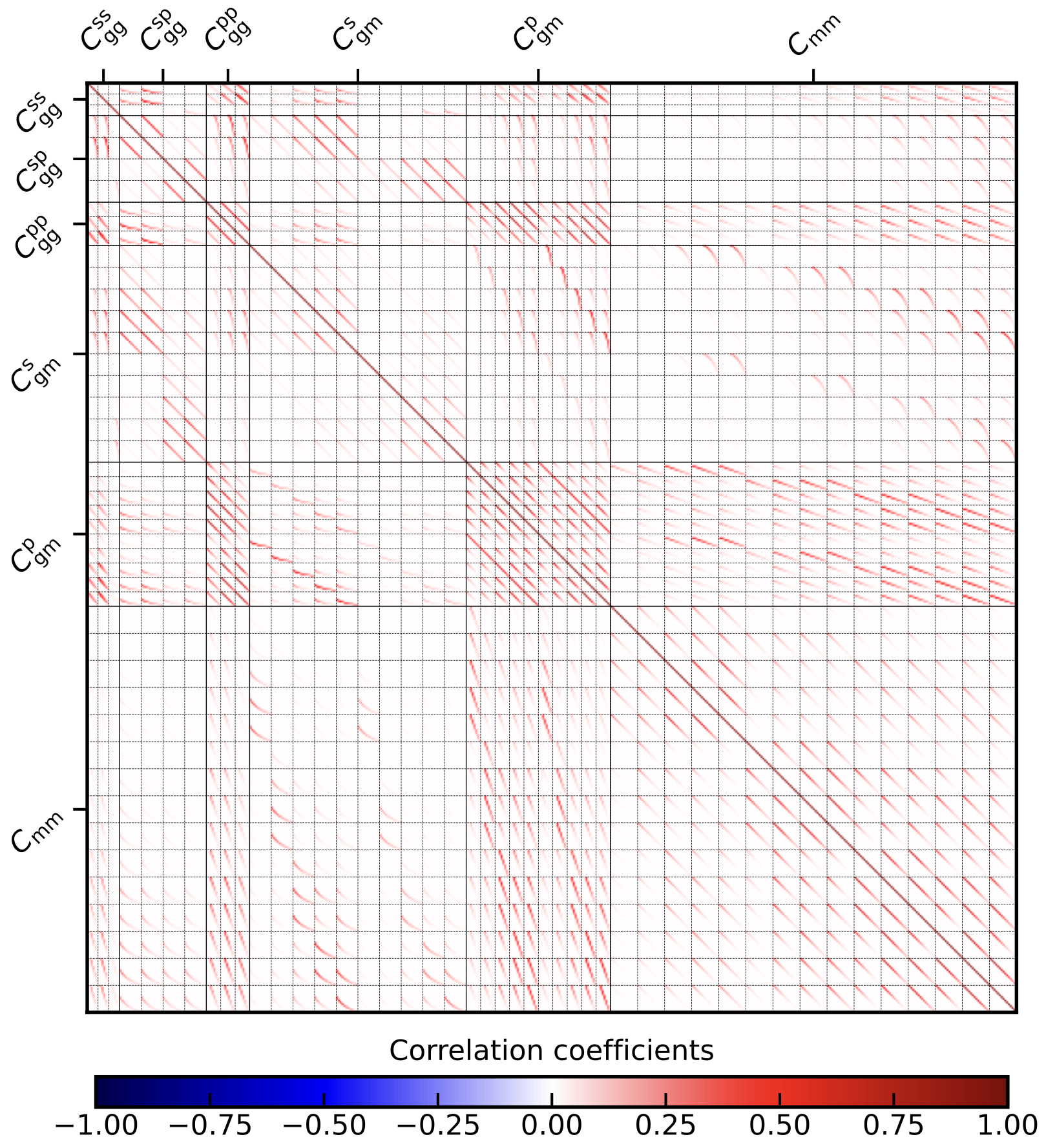
We have three unique combinations of spectroscopic cross spectroscopic bins because we also took the adjacent bin into account. They are binned into six \(\ell\) bins. The spectroscopic cross photometric clustering has four unique bin combinations from the two spectroscopic and two photometric bins and with 12 \(\ell\) bins each. Photometric cross photometric clustering has three unique bin combinations and 8 \(\ell\) bins. Spectroscopic GGL has 10 bin combinations with 12 \(\ell\) bins each and lastly, Photometric GGL has also 10 bin combinations with 8 \(\ell\) bins.

3x2pt analysis and stellar mass function

The file config_3x2pt_pure_Cell_SMF.ini in the directory config_files illustrates how to caclulate the covariance matrix in a \(3\times 2 + 1pt\) analysis, where the 1pt refers the stellar mass function (SMF). To do so, you first need to set

[observables]
cstellar_mf = True

You can then include the settings in the following section

[csmf settings]
csmf_log10Mmin = 7
csmf_log10Mmax = 12.5
csmf_N_log10M_bin = 30
#csmf_log10M_bins =
#csmf_log10M_bins_upper = 10.1, 10.1, 10.1, 10.1, 10.1
#csmf_log10M_bins_lower = 9.1, 9.3, 9.5, 9.7, 9.9
csmf_directory = ./input/conditional_smf/
V_max_file = V_max.asc
f_tomo_file = f_tomo.asc
csmf_diagonal = False

In this case we use 30 bins from \(10^7\,h^{-1}M_\odot\) to \(10^{12.5}\,h^{-1}M_\odot\), logarithmically spaced. Alternatively, you can use csmf_log10M_bins to define the boundaries of the bins if they are non-overlapping, or directly provide the upper and lower limits via csmf_log10M_bins_upper and csmf_log10M_bins_lower respectively. Since the stellar mass function uses the \(V_\mathrm{max}\) estimator, you need to specify a file with the corresponding number of entries for \(V_\mathrm{max}\) which is usually directly estimated from the data. The file f_tomo.asc should contain the fraction of galaxies in each tomographic bin used for the SMF, in our example we only have a single bin. Lastly, csmf_diagonal specifies whether all combinations of tomographic bins (for the SMF) and the stellar mass bins should be calculated. If csmf_diagonal = True, the code only calculates the diagonals, this of course only works if the number of stellar mass bins equals the number of tomographic bins for the SMF. The last question is, how do I specify the latter? You go to the redshift section and set

zcsmf_file = bright_DR4_NS_fluxscale_corrected_nz_LB1.txt
value_loc_in_csmfbin = left

This works in exactly the same way as all other tomographic bins. If you use the SMF, you probably want to use it to constrain the parameters of the HOD, it will therefore be wise to set the mass-range used for the galaxy clustering measurement to the same mass-range over which the SMF is estiamted, therefore, we set in the bias section

log10mass_bins = 7, 12.5

Alternative, you can, similarly to the bins in which the stellar mass function is estimated, set the upper/lower limits here explictely via log10mass_bins_upper and log10mass_bins_lower respectively. In that case, you should remove the log10mass_bins variable from the config file as it is used otherwise. Yo can also ask the code to only consider those tomographic bins for the clustering measurements which directly correspond to the mass bins for the clustering measurement by setting csmf_diagonal_lenses to True. This will therefore only consider the auto-correlations of the tomographic bins used for clustering and the corresponding stellar mass bins. In this case, the number of tomographic bins passed in the redshift section must match the number of stellar mass bins used for the clustering measurement. Running this config file will calculate the previously calcualted \(3\times 2\) covariance, the SMF covariance and their cross-correlations in the following order:

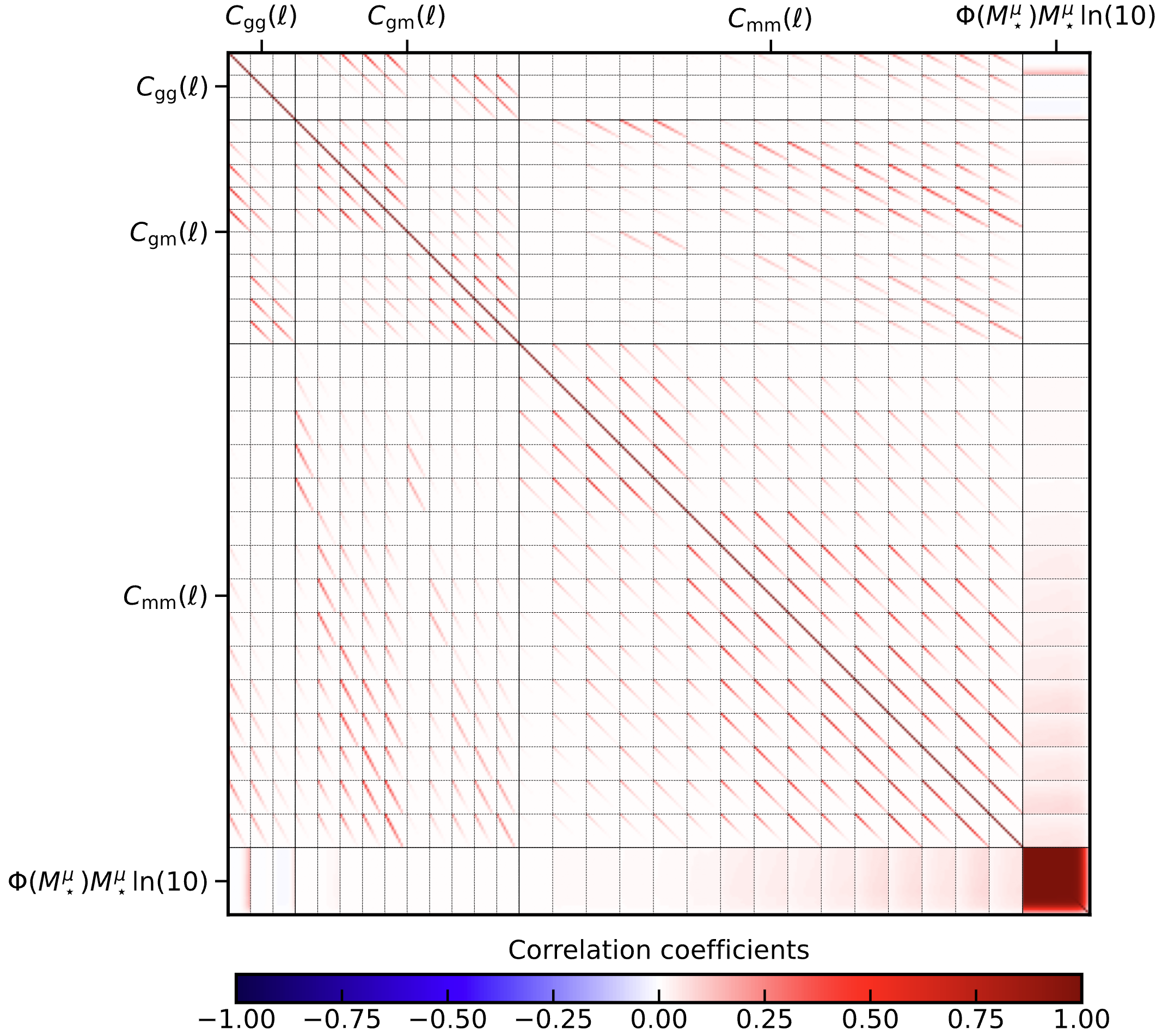
It should be noted, that the SMF is rescaled with the stellar mass and \(\ln(10)\), often the masses are expressed in units of \(h^{-2}M_\odot\), note that the OneCovariance does not do this but uses the standard \(h^{-2}M_\odot\), so remember to convert on input and output.